CNC machines are essential in industries such as aerospace, automotive, and defense, where tool reliability is critical. Predicting tool wear is challenging due to the complex, time-dependent nature of sensor data. These time-series signals often involve nonlinear relationships and dynamic behaviors.
To address this, we propose an efficient deep learning framework combining Long Short-Term Memory (LSTM) networks and Autoencoders (AEs) for tool wear prediction in high-speed CNC milling cutters. The model begins with multi-domain feature extraction and correlation analysis, incorporating features like entropy and interquartile range (IQR), which show strong relevance to tool wear.
Trained on the PHM10 run-to-failure dataset, the LSTM-AE model predicts tool wear values, which are then used to estimate Remaining Useful Life (RUL). The model generally underestimates RUL—favorable for preventive maintenance—and achieves up to 98% prediction accuracy, with improved MAE and RMSE of 2.6 ± 0.3222E-3 and 3.1 ± 0.6146E-3, respectively.Editor
Hamdy K. Elminir, Mohamed A. El-Brawany, Dina Adel Ibrahim, Hatem M. Elattar , E.A. Ramadan
Introduction
The primary objectives of Tool Condition Monitoring (TCM) are categorized into three core functions: fault detection, fault type identification, and Remaining Useful Life (RUL) estimation, the latter also known as prognostics. Unlike traditional detection-focused methods, prognostics aims to predict failures before they occur, marking a significant evolution in predictive maintenance.
Prognostics is broadly defined as any technique that forecasts future system conditions. In particular, it focuses on health assessments by utilizing sensor data to estimate RUL. This typically involves identifying failure indicators, estimating the current system state, and constructing a health index [1,2] .
The main goal of prognostics is RUL prediction—estimating the duration a machine can function safely before failure[3] . In this framework, tool wear is a vital health indicator that directly supports accurate RUL estimation
Data-driven prognostic models operate without prior knowledge of system physics, instead relying on Run-To-Failure (RTF) datasets that represent system performance. In this context, Artificial Intelligence (AI) plays a pivotal role in predictive maintenance, offering capabilities in diagnostics, fault classification, and RUL prediction [4] .
Traditional AI methodologies often employ Machine Learning (ML) techniques, such as Support Vector Machines (SVM) and Random Forests (RF), as well as Deep Learning (DL) strategies.
SVM and RF have been widely adopted for tool wear forecasting and cutter RUL prediction. For instance, RF was used effectively in a study focused on milling tool wear prediction [5] , with comparative evaluations conducted against earlier ML algorithms [6] .
Another notable ML technique, XGBoost, based on gradient boosting, has shown strong performance in RUL estimation for lithium-ion batteries (LIB), especially when hyperparameters were fine-tuned for improved results [7] .
XGBoost has also outperformed traditional regression models in terms of Mean Squared Error (MSE) and Root Mean Squared Error (RMSE) when estimating state of charge in LIBs [8] , and has been applied to battery health assessments [9] .
SVM has also been integrated with Artificial Neural Networks (ANN) and XGBoost in the predictive maintenance (PdM) of chilled beam air conditioning systems [10] . In the Industry 5.0 era, ML approaches have been widely utilized for PdM and Condition Monitoring (CM) [11] .
Among ML models, RF has shown better predictive performance than feed-forward backpropagation (FFBP), while SVM continues to be extensively used in TCM applications [12] .
ANNs remain a central approach in TCM. SVM, RF, and Multi-Layer Perceptron (MLP) models have all been applied to predict and classify tool wear in additively manufactured 316 stainless steel components [13] . ANNs are particularly valued for their robust capabilities in failure analysis, diagnostics, and predictive modeling.
For example, Sindhu, Tabassum Naz et al. introduced an enhanced ANN model for disease diagnostics [14], , while Çolak, Andaç Batur et al. employed ANN combined with Maximum Likelihood Estimation (MLE) to evaluate electrical component reliability [15] .
ANN has also been utilized for modeling breast cancer to predict patient survival [16], and Shafiq, Anum et al. compared ANN with MLE on COVID-19 datasets [17] . In another study [18] , a Rayleigh-distribution-based multilayer ANN, optimized via Bayesian techniques, was developed for estimating reliability parameters.
Additionally, ANN models have been applied to simulate fluid flow behavior, including Ree–Eyring fluids [19] and nanofluids [20,21] . Overall, ANNs have consistently outperformed other models in lifetime reliability analysis [22,23] .
With the rise of Big Data and advancements in sensor technologies, Deep Learning (DL) techniques have become dominant in the prognostics and failure analysis of industrial systems [24] [25] . Among these, Convolutional Neural Networks (CNNs) and Long Short-Term Memory networks (LSTMs) are extensively employed in TCM applications.
CNNs have demonstrated effectiveness in diverse prognostic tasks, such as robotic fuse fault diagnosis [26]and milling tool wear prediction. For instance, a DL model developed in[27]used features derived from force and vibration sensors. This was extended in ) [28] with the Reshaped Time Series Convolutional Neural Network (RTSCNN), which utilized raw sensor data with CNNs as feature extractors. The model included a ReLU-activated dense layer followed by a regression layer to estimate tool wear. Despite its innovations, performance improvements over previous work were minimal.
Hybrid models combining CNN and LSTM architectures have shown promise for tool wear prediction [29]. In [30] , a Convolutional Bi-directional LSTM (CBLSTM) processed raw sensor inputs—CNN extracted local features, which were then passed to BiLSTM units, followed by fully connected layers and a regression output. These models were validated through real-world machining experiments.
Additionally, CNN–LSTM hybrids have been employed to build health indices (HI) and estimate RUL using the C-MAPSS dataset [31] .
LSTM, a specialized form of Recurrent Neural Network (RNN), excels in modeling time-series and sensor data. LSTM has been successfully applied to battery health monitoring and tool wear estimation. For instance, in [32], LSTM combined with Gaussian Process Regression (GPR) created a degradation model using LIB data.
In [33] , a three-phase model integrated XGBoost, a stacked BiLSTM, and Bayesian optimization for battery capacity prediction. LSTM also played a key role in addressing the PHM08 challenge [34] .
A transfer-learning-based BiLSTM model for RUL prediction of rolling bearings was developed in [35]. Broader applications include traffic forecasting using GRU and wavelets [36], and modeling energy consumption in water treatment plants[37] .
LSTM’s effectiveness in tool wear prediction is enhanced by preprocessing strategies. In [38] , it was integrated with Singular Spectrum Analysis and Principal Component Analysis (PCA) to improve dimensionality reduction and feature extraction.
To boost performance, LSTM is frequently combined with CNNs [29] . In [39] , a hybrid CNN–BiLSTM model used a ResNetD structure for final tool wear prediction. Another hybrid in [40] used an attention mechanism to highlight relevant features, achieving strong results across datasets. Similarly, [41] employed a 1D-CNN with residual blocks, feeding outputs into a BiLSTM for wear estimation.
Autoencoders (AEs) are also critical in prognostics due to their ability to extract representative features, denoise data, and model sequential dependencies. In , [42] , an AE combined with the Artificial Fish Swarm Algorithm was used for rotating machinery fault diagnosis. In [43], an improved denoising AE enhanced rolling bearing fault recognition, while [44]presented a sparse stacked AE for analyzing solid oxide fuel cells, showing superior fault diagnosis capabilities.
Due to their ability to reconstruct input signals, AEs are particularly suited for sensor-driven tasks such as those in the PHM10 challenge.
Proposed Model and Methodology
Based on these findings, we propose a hybrid LSTM-AE model for tool wear prediction and precise RUL estimation in CNC milling operations.
Our approach utilizes RTF-based sensor data and evaluates RUL by comparing predicted tool wear with a critical threshold. This strategy has proven highly effective in estimating cutter RUL.
Because the sensor inputs are multivariate time-series data with complex dynamics and autocorrelation, traditional models often struggle. However, AEs handle high-dimensional features through dimensionality reduction, while LSTMs manage sequential dependencies.
To address these challenges, we developed a composite LSTM-AE model and tested it using the PHM10 dataset. The model accurately predicted tool wear and RUL, and its architecture is generalizable to other prognostic applications involving raw sensor data.
Theoretical methodology
∙ Basic LSTM architecture
Recurrent Neural Networks (RNNs) are designed to retain the state of previous cells, making them well-suited for handling sequence-based or time-dependent datasets. During training, the hidden state is updated by combining the state from the preceding time step with the current input, passed through an activation function.
While RNNs are capable of learning both long-term and short-term dependencies in sequential data, they face challenges such as gradient vanishing and exploding problems.
To overcome these limitations, advanced variants like Gated Recurrent Units (GRU) and Long Short-Term Memory (LSTM) networks were introduced.
LSTM networks are specifically designed to capture long-term dependencies through a memory mechanism regulated by a system of gates that control information flow.
An LSTM network consists of a chain of LSTM cells, as illustrated in Fig. 1. Unlike conventional RNNs, LSTM incorporates four network layers (depicted as rectangles in Fig. 1) and uses three types of control gates—forget gate, input gate, and output gate—that work together to manage the memory.
These three gates function as follows:
(1)Forget Gate – ft determines which parts of the previous cell state should be discarded.
(2)Input Gate – it determines which parts of the current input should be used to update the cell state.
(3)Output Gate – selects which information from the cell state will be passed to the output.
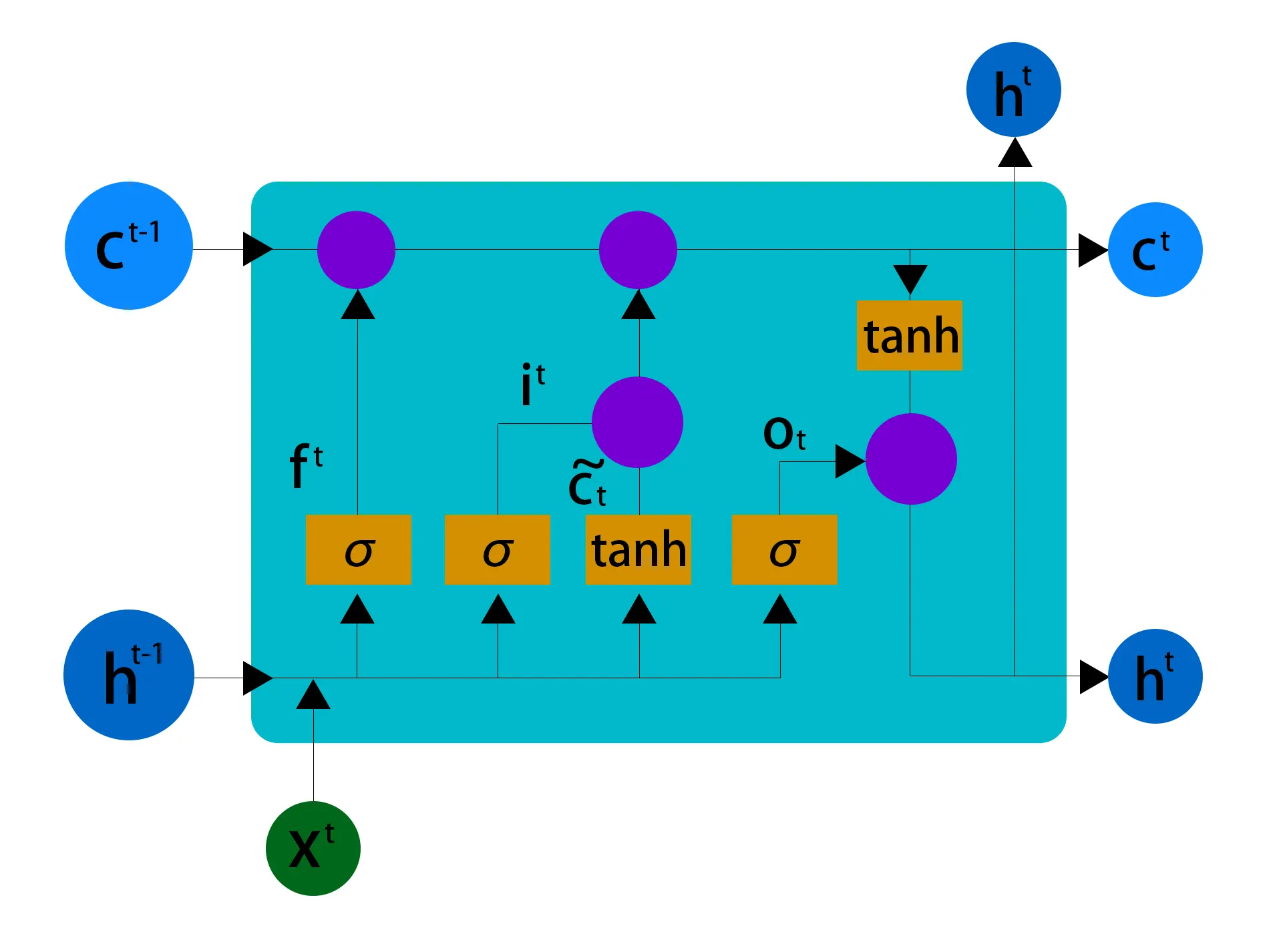
In LSTM, the hidden state ht is updated at each time step t according to the following equations Eq. (1) [46] :

x t is the current data at the same time step, h t-1 is the preceding instant hidden state, the input it, the forget gate ft, 5-the output gate ot and a memory cell ct. Where parameters including all ∈ℝd×k, ∈ℝd×d and ∈ℝd are all learned during network training and are common to all time steps. The last equation gives the hidden layer function ℍ.
The symbol 𝜎(⋅) denotes the logistic activation function, while ⊙ represents the element-wise (Hadamard) product. The parameter 𝑘 is a hyperparameter that defines the dimensionality of the hidden vector.
∙ Auto-Encoder
An Autoencoder is a type of self-supervised learning model designed to learn a compact representation of input data. It has demonstrated strong performance in tasks such as denoising, fault diagnosis, and feature extraction. As illustrated in Fig. 2, an Autoencoder (AE) consists of two main parts: an encoder and a decoder.
The encoder compresses the input data into a latent feature representation, while the decoder takes this encoded information and reconstructs it to approximate the original input.
The input and output layers of the AE have the same number of neurons to ensure accurate reconstruction. For a given input 𝑥∈𝑅𝑚, the operations of the encoder and decoder can be mathematically described as follows [47] :

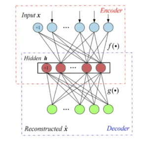
Here, 𝜎, the sigmoid activation function is applied, and ℎ represents the hidden layer output obtained after the encoding transformation. To minimize the error between the input and the reconstructed output, gradient descent is employed, and the corresponding loss function is defined as follows:

where ![]() is the data reconstructed by the decoder.
is the data reconstructed by the decoder.
Methodology
∙ Research motivation
Time-series data involves more complex interrelationships between features compared to single-variable datasets, making feature engineering a challenging task.
While LSTM can effectively capture the dynamic and nonlinear interactions among parameters, the AE neural network excels in learning deep nonlinear relationships between time-series variables.
The LSTM-AE architecture combines the strengths of both LSTM and AE networks. In this model, input data is encoded into fixed-length vectors and then decoded into the desired sequences.
By integrating these two networks, the model can capture the dynamic properties of the input data, making it particularly suitable for industrial processes, such as those involving datasets like PHM10.
∙ Model construction
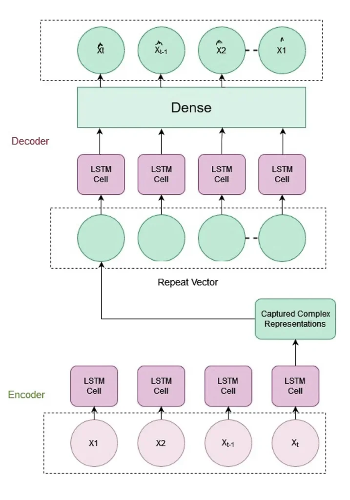
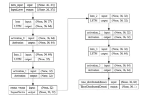
An LSTM-AE model is a hybrid structure that combines LSTM and AE components. It consists of two main parts: an encoder and a decoder, as shown in Fig. 3. The LSTM encoder includes multiple layers of concatenated LSTM cells, which capture long-term dependencies between input features.
The output of the encoding part is an encoded vector, which is then repeated a number of times equal to the timesteps of the LSTM by a RepeatVector component. This repeated vector is fed into the decoder LSTM, which is structured with layers of LSTMs in the reverse order of the encoder, followed by a dense layer and a Timedistributed function to reconstruct the features.
The model’s performance is evaluated based on its ability to reconstruct the input pattern. Once the model achieves satisfactory performance in reproducing the input data, the decoder component may be removed.
In this case, after the model is trained, the reconstruction portion can be discarded, and the model can be used solely for prediction tasks.
While the stacked LSTM is responsible for the prediction process, the ensemble model enhances the accuracy of wear prediction due to its ability to capture long-term dependencies and the most representative features in the encoder section.
Experimental study
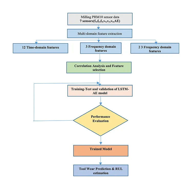
The general framework of the model is illustrated in Fig. 4. It consists of several stages, including feature extraction, selection, model training, and tool wear prediction.
The next section provides a description of the dataset, followed by a discussion of feature engineering, data analysis, and feature selection. Model training and RUL estimation are presented thereafter.
∙ Data description
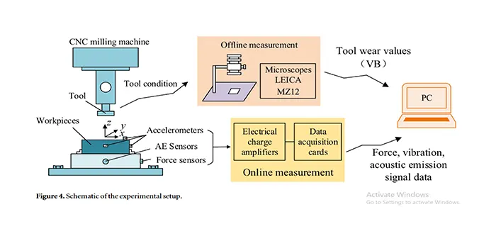
We used the dataset from the PHM10 data competition, which contains data from high-speed CNC milling machine cutters [48]. The dataset includes files for six cutters with three flutes (C1, C2, C3, C4, C5, and C6). Dynamometer, accelerometer, and acoustic emission (AE) sensors were strategically placed to capture data, as shown in Fig. 5.
Data readings from these seven sensors were collected for each of the 315 cuts performed by the cutters, at a rate of 50,000 Hz per channel. Each cutter has 315 independent files corresponding to the 315 runs, with each file structured into seven columns: three-dimensional force (fx, fy, fz), three-dimensional vibration (vx, vy, vz), and AE-RMS (V), representing the acoustic emission signal in RMS value.
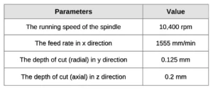
The operational features of the high-speed CNC milling machine being examined are listed in Table 1. Data from C1, C4, and C6 are used for training, testing, and validation, as their wear files are included in the dataset. Each run file is divided into 50 frames, resulting in over 15,000 records for each cutter.
∙ Feature engineering
Researchers often install a dynamometer, accelerometer, and microphone on the machine at strategic locations to capture cutting force, vibration, and acoustic emission data. Previous studies have shown that features from both time and frequency domains can accurately assess tool wear status. In [49] , features extracted from force and vibration sensor readings in different domains were used to detect virtual tool wear.
A health index (HI) was developed in [50] to monitor the tool’s condition using time-frequency domain features from all sensors, extracted through wavelet packet decomposition. Wu et al. [51] also extracted features from various domains and analyzed the correlation between these features using the Pearson Correlation Coefficient (PCC).
The selected features were then input into an Adaptive Neuro-Fuzzy Inference System (ANFIS) for Remaining Useful Life (RUL) prediction of machining tools. PCC was also utilized in [52] for selecting key features for tool wear regression and RUL estimation.
Through a literature review, it becomes clear that multi-domain feature extraction is a crucial step in feature engineering. In our study, we included additional features, such as the interquartile range (IQR) and entropy, in various domains.
IQR is a valuable measure of data spread, helping to identify outliers and the skewness of the dataset. Another important feature is entropy, which quantifies the average amount of “information” or “uncertainty” associated with the potential outcomes of a variable. Both IQR and entropy have shown a strong correlation with tool wear.
Feature extraction, as part of exploratory data analysis (EDA), is a key step in the PHM cycle. These features act as condition indicators that reflect the machinery’s health.
Features can be combined from different domains to form a health index (HI) that expresses the degradation process. Redundant data can introduce noise, negatively affecting model performance. To address this, features with monotonic, trendable, and predictable behaviors should be selected, as discussed below.
We added minimum value, mean value, and IQR to the five-number statistics [53] , along with entropy from the dataset. IQR, which was integrated into the features extracted from the review, is an effective measure of data spread and can identify outliers and skewness.
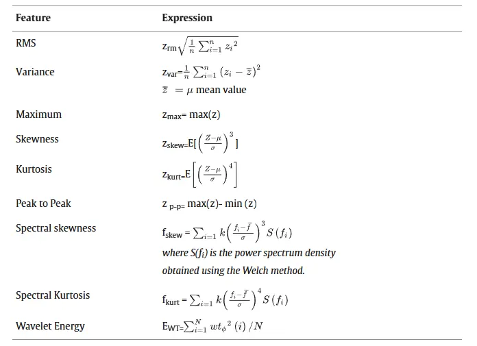
Entropy, which measures the average level of “information” or “uncertainty” in the variable’s possible outcomes, was studied in both time and frequency domains. We extracted the multi-domain features shown in Table 2, including entropy and IQR, using the TSFEL library [54] .
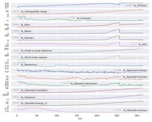
These features were extracted for the seven signals (fx, fy, fz, vx, vy, vz, and AE) from each cutter, and their correlation with tool wear was analyzed to construct the health index for accurate tool wear prediction. Fig. 6 illustrates the extracted features for sensor fx across the entire lifecycle, as an example of the features obtained from RTF.
∙ Data analysis and feature selection
After feature extraction, data analysis is performed to select features that are strongly correlated with wear values, as these serve as health indicators for predicting the target wear value. The Pearson correlation coefficient measures the strength of the relationship between two parameters, indicating how one parameter is affected by changes in the other.
For example, a correlation value of −0.1 indicates a weak negative relationship between variables X and Y, whereas a correlation coefficient of −0.9 would suggest a strong negative relationship.
Principal Component Analysis (PCA) is a technique used to reduce the dimensionality of the dataset, helping to condense the feature space while still effectively representing the data. Many researchers have applied PCA for dataset reduction to express the target variable [55, 56] .
In [57], it was found that about 24 features could explain approximately 98% of the original dataset’s variance. The data is first standardized using the standard scalar formula expressed in Eq. 2, where xmean is the mean value and σ is the standard deviation.
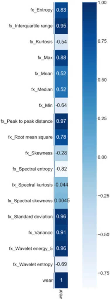
The correlation between features from different signals and the target variable is evaluated using Pearson Correlation Coefficient (PCC) to identify the most relevant features for wear prediction. As shown in Fig. 7, the heatmap illustrates the correlation between wear and various features, helping to select those with the highest correlation.
It is evident that the additional features proposed in this framework, such as entropy and IQR, are significantly correlated with the wear value.
This analysis was also performed for other sensors, such as fy and fz, with similar results regarding the selected features. Some features exhibited inter-correlation, which was taken into account when selecting the feature space.
We reduced the feature space to 6 features per signal, keeping the most correlated ones with the wear signal. Since the Acoustic Emission signal showed a low correlation with the target wear value, it was excluded from the feature space used for training the model.

Where xmean is the mean value and σ is the standard deviation value.
Model training
During the training process, data from C1 and C6 are used for training and validation, while C4 data is utilized for testing the network. A vanilla LSTM model, implemented with a TensorFlow Keras backend, is trained for tool wear prediction and RUL (Remaining Useful Life) estimation.
The model is trained for 700 epochs, with two LSTM layers, two dropout layers, and one dense layer featuring a ReLU activation function. To reduce the time per epoch to 12 seconds, training is conducted using the Google Colab T4 GPU backend.
The tool wear value is predicted, and based on the wear limit, the maximum number of safe cuts (RUL) can be estimated. The trained network parameters are shown in Table 3, and the model’s architecture is illustrated in Fig. 8.

∙ RUL estimation
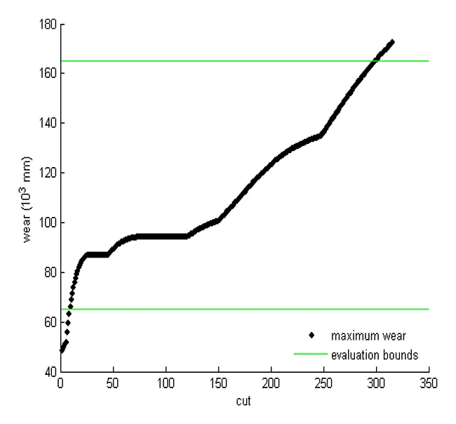
RUL (Remaining Useful Life) refers to the number of cuts a cutter tool can safely make before it reaches complete failure. Using run-to-failure (RTF) data, which spans from the beginning to the point of failure, as shown in Fig. 9, the predicted tool wear values can be combined with the RTF data for RUL estimation, using the algorithm outlined in Table 4.
During the study, it was observed that the first and last few runs contained noisy measurements, so these were excluded, and the wear limit was set to run #300. The PHM Society provided the dataset used in this study as part of the PHM10 competition.

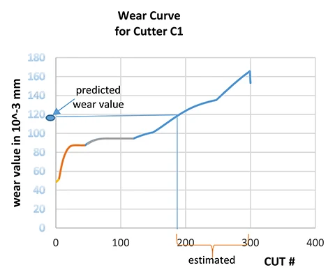
The leaderboard for this competition is available in [58] . After predicting tool wear, the RTF data can be used to estimate the RUL, which represents the number of cuts the tool can safely make before failure, as illustrated in Fig. 10.
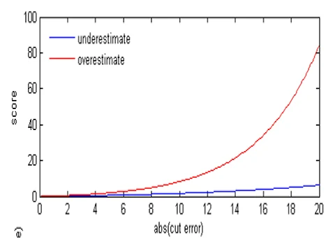
The scoring function used to evaluate the proposed model, which was also employed in the PHM10 competition, is given by Eq. (3). This scoring formula was introduced in [59] . The score achieved by our RUL estimation algorithm was reduced to approximately 40, while the winning score in the PHM10 competition was 5500.

Here, m represents the total number of data points, and di denotes the difference between the predicted RUL (RULˊi) and the actual RUL for each cycle.
The lower the value of this score function, the better the prediction algorithm’s performance. The accuracy of the RUL estimation reaches approximately 99%, with a low score value comparable to the leaderboard results of this competition.
Experimental results
∙ Performance evaluation criteria
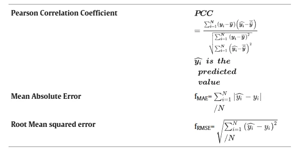
Mean Absolute Error (MAE) and Root Mean Squared Error (RMSE) are the performance metrics used to evaluate the overall efficiency of the proposed LSTM-AE tool wear prediction model. The mathematical formulas for these metrics are provided in Table 5.
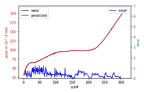
Fig. 11 illustrates the predicted and actual tool wear values for C4, which was used as the test set. After testing the method with the C4 data, the wear curve for other tools or cutters can be forecasted, allowing for RUL estimation of these cutters.
The model can then be applied to estimate the RUL for other cutters as well. The prediction error decreases as the predicted wear values get closer to the actual values, demonstrating that the LSTM-AE model performs effectively within the dimensional criteria used for performance assessment.
∙ Method comparison
Fig. 12 displays the MAE and RMSE values for cutter wear across various methods. The LSTM-AE-based approach is compared with other methods to highlight its effectiveness and advancement.
Conventional intelligence techniques, such as SVR and SVR+KPCA [49], were specifically used for forecasting tool wear. In addition, deep learning methods, including RNN, LSTM, CBLSTM [30], and CNN [60] , were also considered for performance comparison. The results of these comparisons are presented in Table 6.
As shown in Table 6, the SVR algorithm performs poorly when addressing large-scale nonlinear regression problems. Although deep learning techniques like RNN, LSTM, CBLSTM, and CNN can handle nonlinear regression without reducing the feature space, their predicted accuracy still falls short compared to the proposed framework.
Fig. 12. Method Comparison between our LSTM-AE and earlier methods.
| Proposed mehod | MAE(10–3 mm) | RMSE (10–3 mm) |
|---|---|---|
| SVR+PCA [49] | 3.9583±0.9371 | 5.4428±1.5894 |
| RNN [30] | 12.1667±6.2292 | 15.7333±6.2164 |
| SVR [49] | 9.3770±2.0422 | 11.968±3.3337 |
| LSTM [30] | 10.7333±3.8734 | 13.7333±4.5742 |
| CBLSTM [30] | 7.2333±1.0263 | 9.2333±1.9140 |
| CNN [60] | 11.0000±1.3000 | 14.0428±5.5588 |
| Proposed (LSTM-AE) | 2.6 ± 0.3222 | 3.1 ± 0.6146 |
Table 6. Result Comparison.
∙ Result discussion
Fig. 13 presents a comparison between the predicted and actual tool wear values for various cutter cuts throughout their life cycle. The figure highlights the discrepancies between these two values in the shaded areas. Some sections show underestimation, while others show overestimation.
Underestimation occurs when the predicted values are lower than the actual values, resulting in a better performance of the score function. Overestimation is seen when the predicted values exceed the actual tool wear curve. Referring back to Fig. 11, the overall predicted curve tends to underestimate the expected values across the entire curve.
This indicates that the proposed framework’s efficiency in predicting the RUL is lower than the actual values, potentially leading to earlier scheduling of maintenance or component replacement before failure occurs.
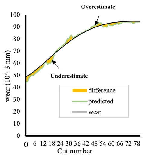
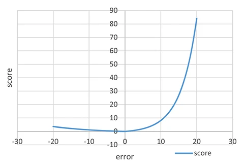
Fig. 14 illustrates the score function [59] . A notable feature of this function is that, in the case of underestimation, the penalty remains nearly constant, meaning the error is lower and the performance is better. This characteristic is evident in the results for the proposed model, as shown in Fig. 15.
∙ Model generalization
The model can be applied to any dataset containing sensor data or a feature map that requires reduction, or even any feature map aimed at predicting the target variable with high accuracy.
If there are specific operating conditions, these can be treated as part of the feature map, or the values of these conditions can be analyzed across different cases to add new columns or features to the dataset.
However, when dealing with very large datasets, the model may encounter computational complexities and redundant information, which could degrade its performance.
This issue can be addressed by incorporating a weighting mechanism for extremely long datasets. This mechanism assigns different weights based on the relevance of the information.
Conclusion
TCM plays a crucial role in industrial processes by focusing on prevention rather than failure detection, ultimately reducing replacement costs and saving lives. Time-series data often involve multiple variables with complex interconnections and dynamic features, which makes traditional TCM particularly challenging, especially when dealing with large sensor datasets. However, deep learning networks such as LSTM and AE show great promise in handling the complexity of these datasets.
As a result, a hybrid deep learning model, LSTM-AE, was developed using an encoder LSTM and an LSTM decoder for tool wear prediction. This model was evaluated for predicting tool wear in CNC milling machine cutters, using the PHM10 original dataset with data from C1, C4, and C6 cutters for training, testing, and validation.
The overall framework consists of several steps: 1) extracting features from different domains of the raw sensor data, 2) performing Pearson correlation coefficient (PCC) analysis to create a feature map that is then input to the LSTM model, and 3) feeding the selected features into the model to predict the target wear.
The study emphasized extracting key features from cutter data, including new ones like IQR and entropy. These features demonstrated a strong correlation with tool wear using PCC, which helped improve model performance.
The proposed framework outperforms previous methods in terms of tool wear prediction accuracy, achieving 98%. It also shows a significant improvement in RMSE and MAE for the test set compared to earlier techniques. By utilizing both the wear threshold and the tool’s degradation curve, the expected wear value is used to estimate RUL, ensuring that RUL values are mostly underestimated, preventing machine failure before it occurs.
The model can be adapted to any dataset with sensor data or feature maps that require reduction, or any feature map aimed at predicting the target variable with high accuracy. However, the model may face computational complexities and redundant data when dealing with very long datasets, which can reduce its performance.
This issue can be addressed by introducing a weighting mechanism for long datasets, assigning different weights based on the value of the information. This approach could open new avenues for research and applications with other datasets. Future research may also focus on developing a multi-objective optimization algorithm to best select the model’s hyperparameters.

